Mangiafico, S.S., County Agent II, Rutgers Cooperative Extension

ABSTRACT

Program evaluation in extension and outreach often relies on the assessment of Likert item data. Appropriate statistical approaches for this task include ordinal regression, traditional nonparametric tests, and aligned rank transformation analysis of variance. Here, these methods are compared for simulated data, and p values, type I errors, and power are presented. t tests and other traditional parametric approaches may be inappropriate for this kind of data. Researchers should not rely on p values as the sole determiner of a meaningful effect. Instead, analysis should also include effect size statistics and an assessment of practical importance.

Introduction

Program evaluation in extension and outreach often relies on the analysis of responses to individual Likert-type questions, or Likert items (Gajda and Jewiss, 2004; Boone and Boone, 2012). These are distinct from Likert scales that are composed of the combined responses to several items such as those commonly used in psychology and sociology (Santos, 1999). To my knowledge, statistical analysis of Likert item data is not typically addressed in analysis of experiments courses or textbooks. Even textbooks covering nonparametric statistics (e.g. Conover, Practical Nonparametric Statistics, 3^rd ed.) or analysis of categorical data (e.g., Agresti, Categorical Data Analysis, 3^rd ed.) may not address Likert item data. Students and faculty accustomed to working with continuous data, classic parametric statistics such as t tests and analysis of variance (ANOVA), and nominal categorical data may be unsure how to approach Likert item data. Questions on analyzing Likert item data are common on websites where students and researchers pose questions about statistical analysis, such as ResearchGate (www.researchgate.net/) and Cross Validated (stats.stackexchange.com/).

 

Methods of Analysis

Descriptors

Likert, statistics, survey, effect size, p value, nonparametric, ordinal regression, aligned ranks

 

Ordinal Data

Likert item data are best viewed as ordinal in nature. The responses from a Likert item are not truly numerical even if the response categories are numbered for convenience. Ordinal data are categorical with the categories being naturally ordered. That is, strongly agree is more positive than agree, and agree is more positive than neutral, and so on.  Representing these categories as e.g. 5, 4, and 3 doesn’t mean that the data are actually numeric.

Treating Likert item data as numeric requires additional assumptions about the spacing of the categories. That is, it may be the case that all the categories are equally spaced and could be converted to numbers such as –2, –1, 0, 1, 2. Or it may be the case that agree is further from neutral than it is from strongly agree. In this circumstance, perhaps the data could be represented as –3, –2, 0, 2, 3. Usually, however, this spacing isn’t known a priori, so that when Likert item data is treated as numeric, an assumption about the spacing of the response categories has been applied implicitly or explicitly.

Treating these data as nominal or unordered categorical is undesirable because the information about the order of the categories is lost. For this reason, a chi-square test of association, for example, may lack statistical power relative to an analysis that includes information on the order of the categories or may answer a question that is not of interest. That is, a chi-square test of association doesn’t account for the fact that strongly agree is more positive than agree, and so on.

Given these considerations, it is often desirable to treat Likert item data as ordinal in nature.

 

Parametric Analysis

For the analysis of Likert item data, Boone and Boone (2012) recommended against using traditional parametric tests like t test, ANOVA, and Pearson correlation in favor of medians, frequencies, chi-square tests, and Kendall correlation. In general, traditional parametric tests may not be appropriate for Likert item data as these data are discrete in nature, usually considered ordinal and not interval, and often do not follow a normal distribution. Practically speaking, there is a worry that using traditional parametric statistics with Likert item data will result in an inflated rate of false-positive results (type I errors), so that reported p values are not reliable.

Inverse normal transformation (INT) is sometimes recommended to convert data from non-normal distributions to a normal one. After transformation, a parametric test can be applied. Luepsen (2018) notes that parametric analysis after INT may behave well with discrete and non-normal data, but Beasley et al. (2018) noted inflated type I error rates with data from some data distributions. This technique would not treat Likert item data as ordinal, and the assumptions of parametric analysis would still need to be met with the transformed data.

 

Traditional Nonparametric Tests

Nonparametric tests overcome these problems by having no assumptions about the distribution of the data, and many of them are applicable for ordinal data. Hollingsworth et al. (2011) recommended using Wilcoxon-Mann-Whitney test (WMW) for Likert item responses from extension surveys. Likewise, analysis methods recommended for Likert item data by Mangiafico (2016) included traditional nonparametric tests such as WMW and Kruskal-Wallis (KW).

One drawback to traditional nonparametric tests is that there are limited experimental designs that can be used with them. For example, KW cannot be used with designs more complex than a one-way design. The Friedman test is applicable only for data arranged in unreplicated complete block design. This excludes more complex designs that include multiple independent variables, interactions, or replicated repeated measures. Additionally, some traditional nonparametric tests require interval data. For example, the Wilcoxon signed-rank test for paired data requires subtraction prior to ranking data. For these tests, assumptions have to be made to convert Likert item data from ordinal to interval.

 

Ordinal Regression

In most cases, ordinal regression (OR) would be an ideal approach for analyzing Likert item data. OR treats the dependent variable as ordinal in nature. In good implementations, OR can be used with complex designs that include interactions, covariates, and mixed-effects models. Various names may be used to describe variants of OR. These include cumulative link model, ordered logit model, and proportional odds model (Christensen, 2018).

In R, the ordinal package (Christensen, 2018) is probably the premier package for OR, and the polr function in the MASS package is also common. In SAS, PROC LOGISTIC will treat a multinomial dependent variable as ordered by default, or PROC GENMOD can be used. In SPSS, PLUM can be used for OR (Tabachnick and Fidell, 2013).

For an experienced user, conducting ordinal regression should be no more difficult than fitting a general linear model. But the process make be somewhat intimidating for novice users, as there is an assumption of proportional odds to be met in the analysis and fitting of some models may fail.

 

Aligned Rank Transformation ANOVA

Aligned rank transformation (ART) ANOVA is a rank-based approach (Wobbrock et al., 2011). In good implementations, it can handle complex designs including interactions and repeated measures. An accessible and relatively easy to use software implementation for R and Windows, ARTool, is presented by Wobbrock, et al. (2018). In ARTool, independent variables in the model can be categorical factors and interactions, but not continuous variables.

One consideration for using ART ANOVA with Likert item data is that the approach—as presented by Wobbrock et al. (2011)—uses cell means and residuals from those means before ranking. This suggests that the dependent variable must be interpreted as being interval in nature. That is, for Likert item data, the researcher must—implicitly or explicitly—make assumptions translating the response categories to numerical values.

With ARTool, I advise users to read carefully the documentation for comparing among interaction effects. Also, Wobbrock et al. (2011) urge caution regarding using this approach when data are extremely skewed, designs are other than completely randomized, or when there are many tied values, as is likely with Likert item data.

While Luepsen (2018) notes that ART is generally considered good when considering type I errors and power for heavy-tailed distributions or distributions with outliers, they also report inflated type I errors in some cases of heteroscedasticity, unequal sample sizes, strongly skewed distributions, and discrete values.

 

Comparison among Methods

OR could be considered a standard approach for analyzing Likert item data. But for the sake of simplicity and familiarity, researchers may want to employ traditional nonparametric tests or ART ANOVA. Table 1 summarizes some advantages and disadvantages of approaches to analyzing Likert item data.

 

Table 1. Advantages and Disadvantages of Approaches to Analyzing Likert Item Data

Approaches	Examples	Scales of dependent variable	Advantages	Disadvantages
Ordinal regression	Ordinal package and MASS:polr function in R PROC LOGISTIC and PROC GENMOD in SAS PLUM in SPSS	Ordinal	Flexible designs including interactions, covariates, and repeated measures	May be somewhat difficult for inexperienced users Fitting of models may fail, and other assumptions need to be met
Traditional nonparametric tests	Wilcoxon-Mann-Whitney Kruskal-Wallis Wilcoxon signed-rank Friedman	Ordinal for most; interval for some	Relatively easy Relatively familiar to audience	Limited designs exclude interactions and most repeated measures
Aligned rank transformation ANOVA	ARTool package in R ARTool software for Windows	Interval for ARTool	Flexible designs including interactions and repeated measures	May be somewhat difficult for inexperienced users Does not allow continuous independent variables Caution is encouraged if data distributions are strongly skewed, heterogeneous, of unequal sample size, or discrete (such as Likert item)

 

 

Comparison of Methods with Simulated Data

I compared results of Wilcoxon-Mann-Whitney (WMW), two-sample aligned rank transformation (ART) ANOVA, t tests, and t tests after inverse normal transformation (INT) to those from ordinal regression (OR). Data were simulated for 5-point Likert item data with 25 observations per sample, drawn from different distributions. It is important to note that the simulated results may not be representative of other situations—for example, when more than two samples are compared, when sample sizes are small or unequal, or when other designs are used.

The type I error rate was the proportion of tests finding a significant difference between samples when the samples were in fact selected from the same distribution. Given the traditional alpha of .05, the type I error rate should be about .05. The type II error rate was the proportion of tests failing to find a significant difference between samples when the samples were in fact selected from different distributions. Power was calculated as 1 minus the type II error rate. The power for these simulations was relatively low, as some distinct distributions from which samples were drawn were relatively similar and the sample size was not particularly large.

Figures 1 and 2 suggest that results for WMW and ART ANOVA were in general agreement with those from OR for the conditions of the simulation. The trend of points falling above the 1-to-1 line in the region of p = .05 suggests WMW and ART ANOVA were less likely to find significant differences in marginal cases when compared with OR.

 

 

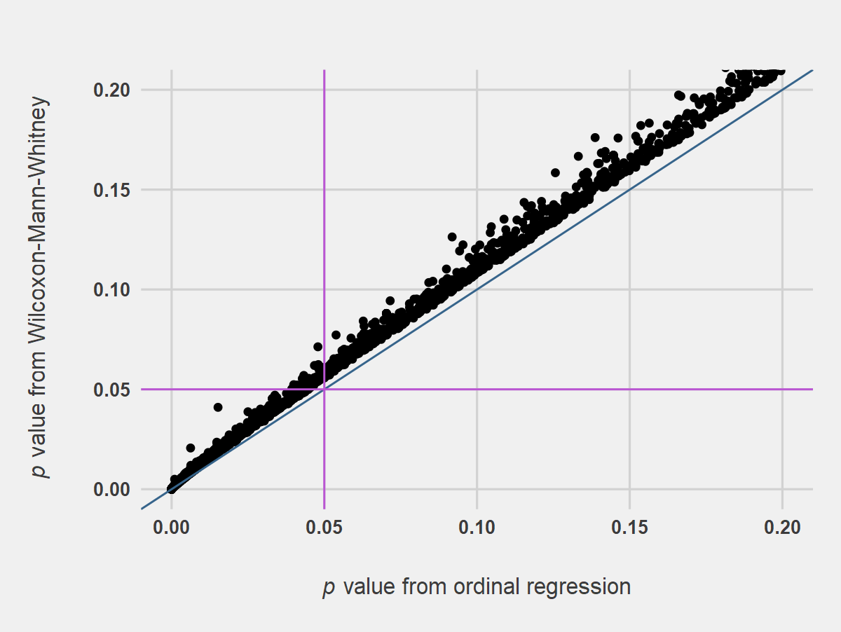
Figure 1. Simulated p Values from Wilcoxon-Mann-Whitney Tests Compared with p Values from Ordinal Regression. Notes for Figure 1: Analysis was on two-samples, 5-point Likert item data, n = 25 per sample, 10,000 replications. The blue line indicates the 1-to-1 line, and the orchid lines indicate p values of .05. Adapted from Mangiafico (2016).

 

 

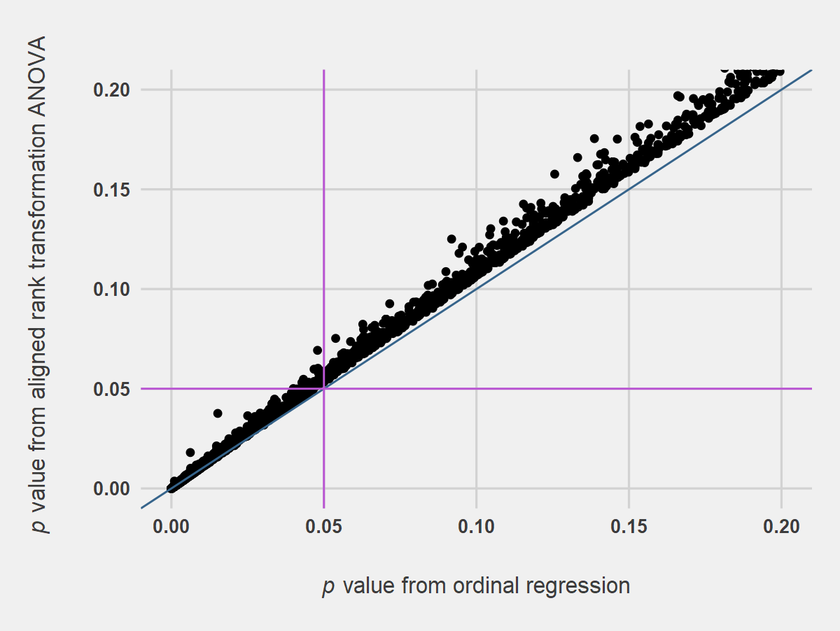
Figure 2. Simulated p Values from Aligned Rank Transformation ANOVA Compared with p Values from Ordinal Regression. Notes for Figure 2: Analysis was on two-samples, 5-point Likert item data, n = 25 per sample, 10,000 replications. The blue line indicates the 1-to-1 line, and the orchid lines indicate p values of .05. The aligned rank transformation ANOVA assumed equal spacing of the Likert response categories.

 

Comparisons of type I error rates and power across the methods suggest that WMW and ART ANOVA were similar or slightly more conservative in type I error rates than OR, and that power among WMW, ART ANOVA, and OR were similar for the conditions of the simulation (Table 2). These results generally agree with those of de Winter and Dodou (2010) and Derrick and White (2017), whose simulations showed that both WMW and Student’s t test were relatively conservative with type I errors when used to compare two samples of 5-point Likert item results.

 

 

Table 2. Summary Results of Simulations Comparing Ordinal Regression, Wilcoxon-Mann-Whitney, Aligned Rank Transformation ANOVA, and t Test

Approach	Type I error rate	Type II error rate	Power
Ordinal regression	.051	.29	.71
Wilcoxon-Mann-Whitney	.046	.30	.70
Aligned rank transformation ANOVA	.048	.29	.71
Welch’s t test	.046	.29	.71
Student’s t test	.045	.24	.76
Welch’s t test on inverse normal transformed values	.049	.25	.75

Notes for Table 2: Analysis was on two-samples, 5-point Likert item data, n = 25 per sample, 10,000 replications. The aligned rank transformation ANOVA and t tests assumed equal spacing of the Likert response categories.           

 

Figure 3 shows the results of Welch’s t tests compared with OR. The plot indicates quite a bit of scatter about the 1-to-1 line in the region of p = .05 and throughout the plot, suggesting that t test may not be a suitable substitute for OR. This is likely to be the case particularly if distributions are strongly skewed. The effect of scatter in the plot is less than appears, however, as 97.8% of t tests in the simulation agreed with the results from OR (alpha = .05). Results from Student’s t tests were visually similar (data not shown). Figure 4 shows somewhat less scatter when INT values were used in t tests, and 99.1% of INT t tests in the simulation agreed with the results from OR (alpha = .05).

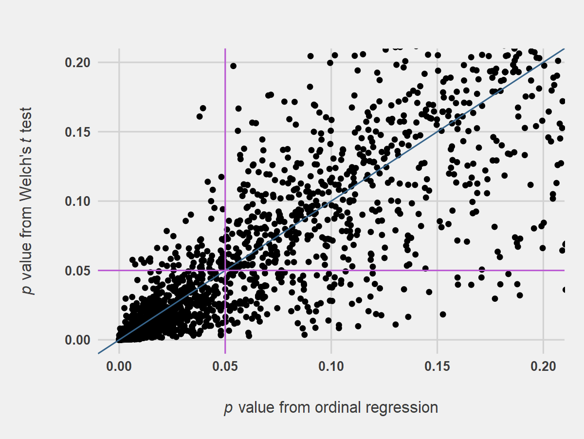
Figure 3. Simulated p Values from Welch’s t tests Compared with p Values from Ordinal Regression. Notes for Figure 3: Analysis was on two-samples, 5-point Likert item data, n = 25 per sample, 10,000 replications. The blue line indicates the 1-to-1 line, and the orchid lines indicate p values of .05. The t tests assumed equal spacing of the Likert response categories.

 

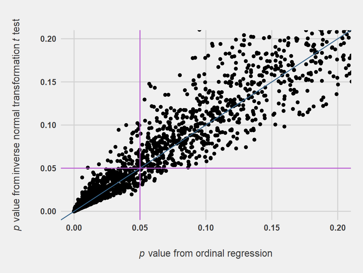
Figure 4. Simulated p Values from Welch’s t tests on Inverse Normal Transformed Values Compared with p Values from Ordinal Regression. Notes for Figure 4: Analysis was on two-samples, 5-point Likert item data, after an inverse normal transformation was applied, n = 25 per sample, 10,000 replications. The blue line indicates the 1-to-1 line, and the orchid lines indicate p values of .05.

 

Conclusions for Comparing Methods

The results described here suggest that for the narrow conditions of the simulations, traditional nonparametric tests and ART ANOVA are reasonable substitutes for OR. Both WMW and ART ANOVA were conservative with type I errors and similarly powered to OR. These results suggest that OR, traditional nonparametric tests, and ART ANOVA may be appropriate approaches for analyzing Likert item data.

t tests may not be appropriate for analyzing Likert item data for theoretical reasons, especially if the data are treated as ordinal or the distribution of values deviates strongly from a normal distribution. The simulations described here show that the p values from t tests will deviate largely in some cases from those from more appropriate tests such as OR. In this respect, INT improved the results of t tests somewhat.

 

p Values, Effect Sizes, and Practical Importance

Researchers evaluating extension and outreach programs typically approach statistical analysis by calculating p values for hypotheses following the null hypothesis significance testing (NHST) framework. This framework is a combination of the ideas of Jerzy Neyman and Egon Pearson and of Ronald Fisher in the 20^th century (Perezgonzalez, 2015). The use of NHST has been controversial, sometimes due to inherent tensions within the method itself, but often due to its application by users who may misunderstand what conclusions can be drawn from the results. In particular, researchers may place undue emphasis on a p value cutoff of .05, arriving at an entirely different conclusion for a p value of .049 than for a p value of .051. A common misconception is that a statistically significant result implies a practically meaningful or important result. A third consideration is that researchers may fail to appreciate that when there are multiple hypothesis tests, a significant result may be likely for at least one test just due to chance.

In response to criticism of the NHST approach, the American Statistical Association (ASA) released a statement on the use of p values (Wasserstein and Lazar, 2016; Wasserstein, 2016). In this statement, the ASA recognized the utility of p values for providing evidence against a null hypothesis but criticized how p value results are sometimes interpreted. They critiqued the common practice of using a threshold value, typically alpha = .05, to distinguish significant effects from non-significant effects. They also recommended full reporting, transparency, and integrity, urging researchers to avoid cherry picking, p value hacking, and data dredging. They also emphasized that statistical significance does not entail scientific, human, or economic importance.

 

Sample Size Affects p Values

An important property of p values is that they are affected by the sample size of a study. As the sample size increases, smaller p values are likely to be produced for an effect of a given size. As a demonstration of this property, consider two examples of hypothetical responses from a single Likert item. For convenience, 1 is used to represent very unlikely, 2 for unlikely, and so on.

For Example 1, we have eight respondents, and WMW indicates a p value of .054.

Example 1

     Group A = 1, 2, 2, 3, 3, 3, 3, 4

     Group B = 2, 3, 3, 4, 4, 4, 4, 5

     p = .054

For Example 2, if we keep the distribution of values exactly the same but double the observations, the p value would decrease to .005.

Example 2

     Group A = 1, 2, 2, 3, 3, 3, 3, 4,   1, 2, 2, 3, 3, 3, 3, 4

     Group B = 2, 3, 3, 4, 4, 4, 4, 5,   2, 3, 3, 4, 4, 4, 4, 5

     p = .005

If we were using alpha = .05 for a cutoff of significance, we would come to different conclusions for Example 1 and Example 2, even though these examples have the same distribution of values in the groups.

This effect is a feature of p values, and not inherently problematic. But it does suggest that for relatively large sample sizes, a significant p value may be reported for a small effect, perhaps an effect too small to be of practical importance. This consideration supports the conclusion that p values should not be relied on as the sole determiner of whether an effect is meaningful.

 

Summary Statistics to Indicate the Size of an Effect

Reporting summary statistics and using plots can be helpful to convey the size of an effect. For example, the median values for the groups in the hypothetical examples above are neutral (3) and likely (4), respectively. The author or reader would need to judge whether the difference in these medians from a 5-point Likert item is a meaningful difference. A bar plot of results for these examples show that the distributions of the two groups are similar in shape, but with Group A centered on a value of 3 and Group B centered on a value of 4 (Figure 5). Because the y-axis is labeled with percentages and not counts, this figure could represent data from either Example 1 or Example 2.

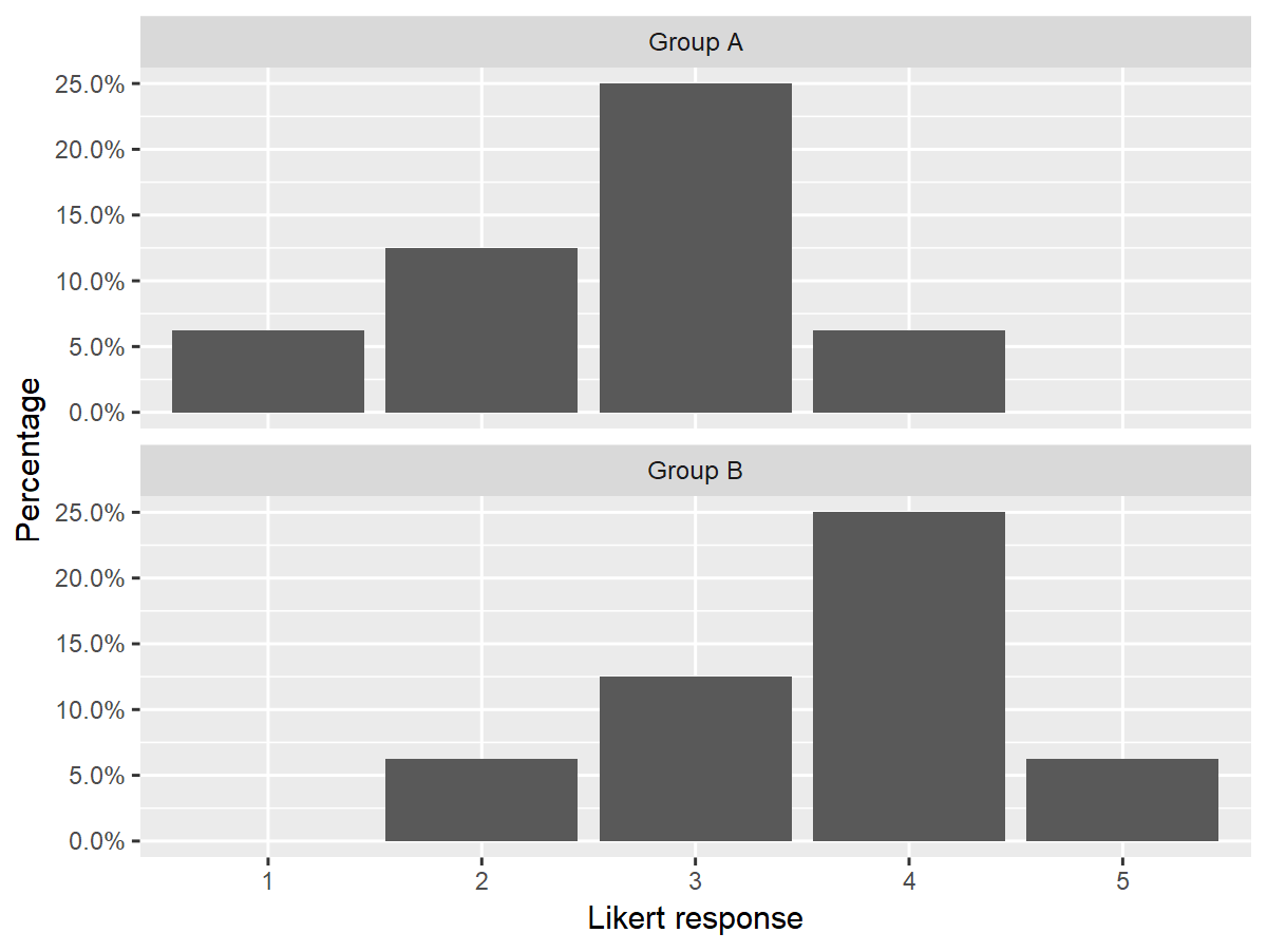
Figure 5. Bar Plots for Frequencies of Hypothetical Likert Item Responses for Two Groups.

Reporting summary statistics to indicate the size of an effect is most useful if the units are understood by the reader. For example, if a treatment increased corn yield 25 bushels per acre, this information would likely be meaningful to an agronomist, but other readers may benefit from having the result expressed in another way.

 

Effect Size Statistics

Effect size statistics report effect sizes in a standardized way so that they are not affected by sample size or measurement units. They are often formulated to vary from 0 to 1, or from –1 to 1. Some effect size statistics have standard interpretations for “small,” “medium,” and “large” effects, although it is important to recognize that these interpretations are always relative to the field of study and specific application and cannot be considered universal or definitive. Cohen (1988) is a source for some effect size statistics and their interpretations. Table 3 lists some common effect size statistics corresponding to certain statistical tests.

 

 

Table 3. Some Common Effect Size Statistics

Statistical test	Corresponding effect size statistic
t test paired t test one-sample t test	Cohen’s d
Analysis of variance  (ANOVA)	eta2 partial eta2 omega2
Wilcoxon-Mann-Whitney	Cliff’s delta Vargha and Delaney’s A
Kruskal-Wallis	epsilon2 Freeman’s theta
chi-square test of association	Cramér’s V phi
Pearson correlation	r
Linear regression	r2

 

Vargha and Delaney’s A (VDA) is an appropriate effect size statistic to use with WMW. It reports the probability of an observation in one group being larger than an observation in the other group. A probability of .5 means that the groups are stochastically equal, whereas probabilities close to 0 or 1 reflect the result that an observation from one group is likely to be larger than an observation from the other group. Vargha and Delaney (2000) give interpretations for values for VDA (Table 4).

 

Table 4. Interpretation for Vargha and Delaney’s A (VDA)

VDA	Interpretation
.00  –     .29	Large
> .29  –     .44	Medium
> .44  –  < .56	Small
.56  –  < .71	Medium
.71  –   1.00	Large

 

For the hypothetical examples discussed above, VDA = .78. This result is the same for both Example 1 and Example 2. The standard interpretation for this probability would be that this is a large effect size. That is, that the probability of an observation in Group B being greater than that for Group A is considered large, regardless of the calculated p value.

One advantage of effect size statistics is that the reader does not need to understand the measurement units used (Grissom and Kim, 2012). Likewise, effect size statistics can be used to compare effects across studies that used different units but comparable effect size statistics (Grissom and Kim, 2012).

It should be remembered that standard interpretations of effect sizes may not be appropriate in all cases. For example, in matters of life and death, large sums of money, or activities repeated many times, small effect sizes can have great practical importance.

 

Practical Importance

Ultimately, neither p values nor effect size statistics can replace human understanding of the context in which research is conducted. Drawing conclusions from experimental results often includes economic, social, moral, and practical considerations.

 

General Conclusions

As it is desirable for theoretical and practical reasons to treat Likert item data as ordered categorical data, ordinal regression could be considered an ideal approach for analysis due to its flexibility; however, for simple designs, traditional nonparametric tests might be preferable due to their simplicity and familiarity.

In conducting statistical analyses, researchers are encouraged not to rely solely on p values to determine the importance of statistical findings and not to place undue emphasis on the alpha = .05 threshold for statistical significance. One should remember that a significant p value does not imply a large effect or a practically meaningful effect. Summary statistics, plots, effect size statistics, and practical considerations are important in assessing results and conveying results to readers.

 

References

Beasley, T.M., Erickson, S., and Allison, D.B. (2009). Rank-based inverse normal transformations are increasingly used, but are they merited? Behavior Genetics, 39(5) 580–595.

Boone, H.N., and Boone, D.A. (2012). Analyzing Likert data. Journal of Extension, 50(2), Article 2TOT2. Available online: www.joe.org/joe/2012april/tt2.php

Christensen, H.R.B. (2018). Cumulative link models for ordinal regression with the R package ordinal. Vienna, Austria: The Comprehensive R Archive Network. Available online: cran.r-project.org/web/packages/ordinal/vignettes/clm_article.pdf

Cohen, J. (1988). Statistical power analysis for the behavioral sciences (2nd ed.). Hillsdale, NJ: Lawrence Erlbaum Associates.

Derrick, B., and White, P. (2017). Comparing two samples from an individual Likert question. Journal of Mathematics and Statistics, 18(3), 1–11.

Gajda, R., and Jewiss, J. (2004). Thinking about how to evaluate your program? These strategies will get you started. Practical Assessment, Research, & Evaluation, 9(8) 1–7. Available online: PAREonline.net/getvn.asp?v=9&n=8

Grissom, R.J., and Kim, J.J. (2012). Effect sizes for research : univariate and multivariate applications. Routledge.

Hollingsworth, R.G., Collins, T.P., Easton Smith, V., and Nelson, S.C. (2011). Simple statistics for correlating survey responses. Journal of Extension, 49(5), Article 5TOT7. Available online: joe.org/joe/2011october/tt7.php

Luepsen, H. (2018). Comparison of nonparametric analysis of variance methods: a vote for van der Waerden. Communications in Statistics - Simulation and Computation, 47(9) 2547–2576.

Mangiafico, S.S. (2016). Summary and analysis of extension program evaluation in R (v. 1.15). New Brunswick, NJ: Rutgers Cooperative Extension. Available online: rcompanion.org/handbook/

Perezgonzalez, J.D. (2015). Fisher, Neyman-Pearson or NHST? A tutorial for teaching data testing. Frontiers in Psychology, 6, 223.

Santos, J.R.A. (1999). Cronbach’s alpha: a tool for assessing the reliability of scales. Journal of Extension, 37(2), Article 2TOT3. Available online: www.joe.org/joe/1999april/tt3.php

Tabachnick, B.G., and Fidell, L.S. (2013). Using multivariate statistics (6th ed.). Upper Saddle River, NJ: Pearson Education.

Vargha, A., and Delaney, H.D. (2000). A critique and improvement of the CL common language effect size statistics of McGraw and Wong. Journal of Educational and Behavioral Statistics, 25(2), 101–132.

Wasserstein, R.L., and Lazar, N.A. (2016). The ASA’s statement on p-values: context, process, and purpose. American Statistician, 70(2), 129–133.

Wasserstein, R. (2016, March 7). American Statistical Association releases statement on statistical significance and p-values: Provides principles to improve the conduct and interpretation of quantitative science. ASA News.

de Winter, J.C.F., and Dodou, D. (2012). Five-point Likert items : t test versus Mann-Whitney-Wilcoxon. Practical Assessment, Research & Evaluation, 15(11), 1–16. Available online: pareonline.net/getvn.asp?v=15&n=11

Wobbrock, J.O., Findlater, L., Gergle, D., and Higgins, J.J. (2011). The aligned rank transform for nonparametric factorial analyses using only anova procedures. In Conference on Human Factors in Computing Systems (pp. 143–146).

Wobbrock, J.O., Findlater, L., Gergle, D., Higgins, J.J., and Kay, M. (2018). ARTool: align-and-rank data for a nonparametric ANOVA. University of Washington. Available online: depts.washington.edu/madlab/proj/art/index.html

---